Introduction

The Three Pillars of Observability—logging, metrics, and tracing—help you better understand how your system works. They provide a complete picture of your systems' health, performance, and actions. In this article, we will explore how to implement these three concepts in a distributed system composed of multiple technologies. There are several tools and frameworks available for this purpose; in this tutorial, we will use the tools provided by the ELK stack.

Let's begin by visualizing our target system with a diagram. In the following illustration, we can see that our system consists of two distinct REST APIs and one database. It's important to understand that these components are separate applications, each with its own unique characteristics. To demonstrate the interoperability of the solution, the order service is coded in Java, while the shipping service is coded in Python. All communication between these applications is facilitated through REST APIs.

In a distributed system like this, composed of multiple technologies, it becomes essential to have a comprehensive understanding of the system's health, performance, and actions. By implementing the three pillars of observability, we can achieve this level of insight and ensure the smooth functioning of the entire system.

To accomplish this task, we will utilize Elastic, Logstash, and Kibana and APM, these tools, when combined, provide us with the necessary means to monitor our system end-to-end.
Elastic, the search and analytics engine, allows us to efficiently store, search, and analyze large volumes of data in real-time. Logstash, a data processing pipeline, helps us collect, parse, and transform logs from various sources before sending them to Elastic. APM is an application performance monitoring system built on the Elastic Stack. It allows you to monitor software services and applications in real time, by collecting detailed performance information on response time for incoming requests, database queries, calls to caches, external HTTP requests, and more. (Reference)
Kibana, a data visualization and exploration tool, enables us to create dynamic dashboards and visualizations that offer valuable insights into the system's health, performance, and actions.

By utilizing these tools, we can effectively implement the three pillars of observability.

Before jumping into the code let's define some concepts.

Logs

Logs are time-stamped text records of events that happen within a system. They provide a chronological account of what happened, when it happened, and where it happened. Logs can include information like user activities, system events, errors, and diagnostic data.

Metrics

Metrics are numerical values that represent the state of a system at a specific point in time. They are commonly used to monitor and measure the performance and health of a system. Examples of metrics include response times, memory usage, CPU load, error rates, and more. These metrics can be continuously analyzed to track trends, identify potential issues before they escalate, and make informed decisions about system optimization and capacity planning.
For example, we can use the CPU load metric to trigger a autoscaling event.

Traces

Traces provide a detailed picture of how a transaction or request moves through a system, even if this system is composed by multiple independent applications.
They help to understand the journey of a request, from the moment it starts being processed until the response is returned to the client.

Objectives

Let's first define some objectives for the next sections:

Create the Orders Service and Shipping service as we saw in the previous diagram
Log all the relevant information and export the logs to Elastic
Export system performance metrics to Elastic
Export business oriented metrics to Elastic
Export traces to Elastic

In summary, once everything is configured, our system will consist of two APIs and one database. We will use Kibana for analyzing logs, metrics, and traces, and build dashboards to provide a precise picture of our system's working condition.

Create the APIs

💡

You can find the full source code and a docker compose file with the ELK stack in GitHub. In this post we won't deep dive into the details of each API.

For this demo, we can simply start everything using the Docker Compose file present on Github.

docker compose build
docker compose up -d

You can launch all the containers by running docker compose build and docker compose up -d

Once all the containers are up and running, you should be able to access localhost:8080/products and see a list of products. Invoke this endpoint several times to generate some logs. For now, you can view them in the Docker logs, but we'll soon explore how they are sent to Elasticsearch and how to access them through Kibana.

LOGS

Logs, the first pillar, are something everyone should be familiar with, ranging from the most basic System.out.println to more advanced logging frameworks like logback or log4j. Occasionally, everyone needs to send something to the console output, whether it's to detect an annoying bug or to monitor the progress of a method, we all been there.

@GetMapping
public ResponseEntity<List<ProductDTO>> getAllProducts() {
    LOGGER.info("Requested the list of products");
    List<ProductDTO> products = productService.getAllProducts();
    LOGGER.debug("Returned {} products to the customer", products.size());
    return ResponseEntity.ok(products);
}

The code snippet above demonstrates a typical log statement in Java. Here, we use the SLF4J facade with Logback, but any other logging library could be used. The output for this is quite straightforward; when the method is invoked, it logs two statements: one at the info level and another at the debug level.

2024-01-20 20:17:08 [http-nio-8080-exec-2] INFO  c.h.a.d.o.ProductController - Requested the list of products
2024-01-20 20:17:08 [http-nio-8080-exec-1] DEBUG c.h.a.d.o.ProductController - Returned 10 products to the customer

This approach is effective for local development; however, a more robust logging strategy is necessary for a real application used by hundreds of users simultaneously. Asking the developers to connect to the server and read the log file each time they need to review the application logs is not a practical solution. Consider a scenario where there are 10 replicas of the application running simultaneously. In such a case, managing and monitoring logs across all instances becomes increasingly complex and time-consuming.

To address this issue, it is essential to implement a centralized logging system that aggregates logs from all application instances and makes them easily accessible for developers, or others stakeholders. This way, they can efficiently analyze and troubleshoot issues in the production environment.

For this job, we'll use Elastic, Logstash, and Kibana.

💡

In fact we will skip Logstash on this demo. We won't do any processing/transformation to the logs. We can send them directly to ElasticSearch

elk stack logs flow until kibana

Log Files

As the name suggests, these are simply files containing logs. However, we need to make a decision about the log format. As seen earlier, our console logs appear like this:

2024-01-20 20:17:08 [http-nio-8080-exec-2] INFO  c.h.a.d.o.ProductController - Requested the list of products
2024-01-20 20:17:08 [http-nio-8080-exec-1] DEBUG c.h.a.d.o.ProductController - Returned 10 products to the customer

We could use this format, but we would need to create custom parsing rules for Logstash to process them. For instance, we would have to instruct Logstash which parts of the string represent the log level, the message, the timestamp, and so on. This strategy also makes log ingestion quite fragile; if a developer changes the format of the log line, the ingestion pipeline could stop working.

However, there is an alternative method for sending and storing logs: using JSON, specifically in the Elastic common schema format(ECS). By adopting ECS, our previous log lines become:

{
  "@timestamp": "2024-01-20T20:34:20.234Z",
  "log.level": "DEBUG",
  "message": "Returned 10 products to the customer",
  "ecs.version": "1.2.0",
  "process.thread.name": "http-nio-8080-exec-1",
  "log.logger": "com.hugomalves.apm.demo.ordersservice.ProductController"
.....
... More information can be added as needed
}

This format is much more friendly for the parsers, all the info is correctly organized in the JSON document. However it is not so user friendly, that's why it should only be used for the logs we export to Elastic, for the local development, we keep using the console format. You should configure your application's log framework to adopt this behavior. The APIs provided on the Github repository already adopt this behavior.

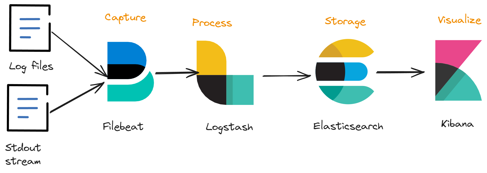
If you explore the docker compose file you will see a service called filebeat. This service is responsible to read the log files created by the APIs and sending them to Elastic. Although it is not within the scope of this post, it is essential to understand its role in the process.

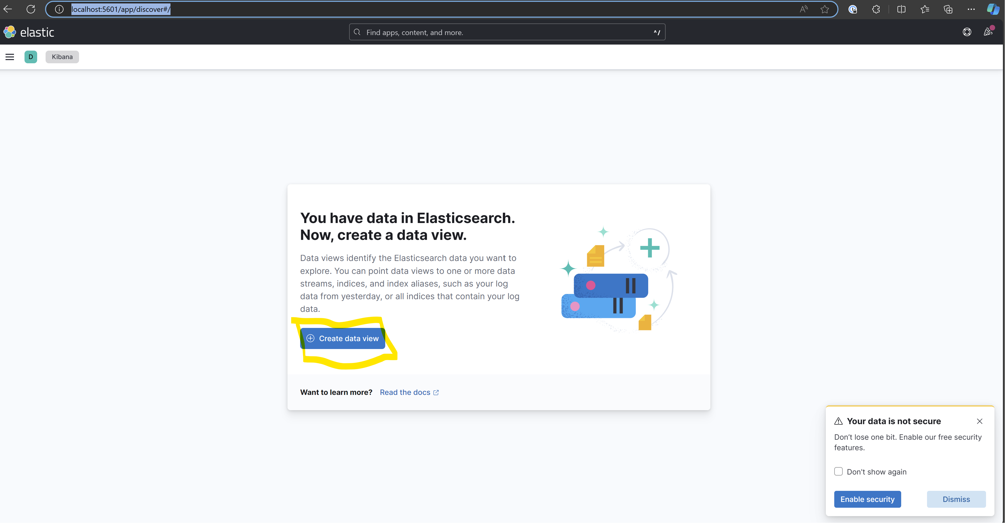
Once all the services defined in the compose file are up and running, navigate to Kibana: http://localhost:5601/app/discover#/ and create the log index. (Although outside the scope of this post, this index is specific to Kibana. Other tools may not have this concept, but you can learn more about indexes here.)

💡

Before moving forward check if all the containers are running

Open the page and click on "Create Data View"

kibana create index

Name your new index, and specify the pattern. You can name it as you want, however the pattern must be named "filebeat*".

kibana create data view

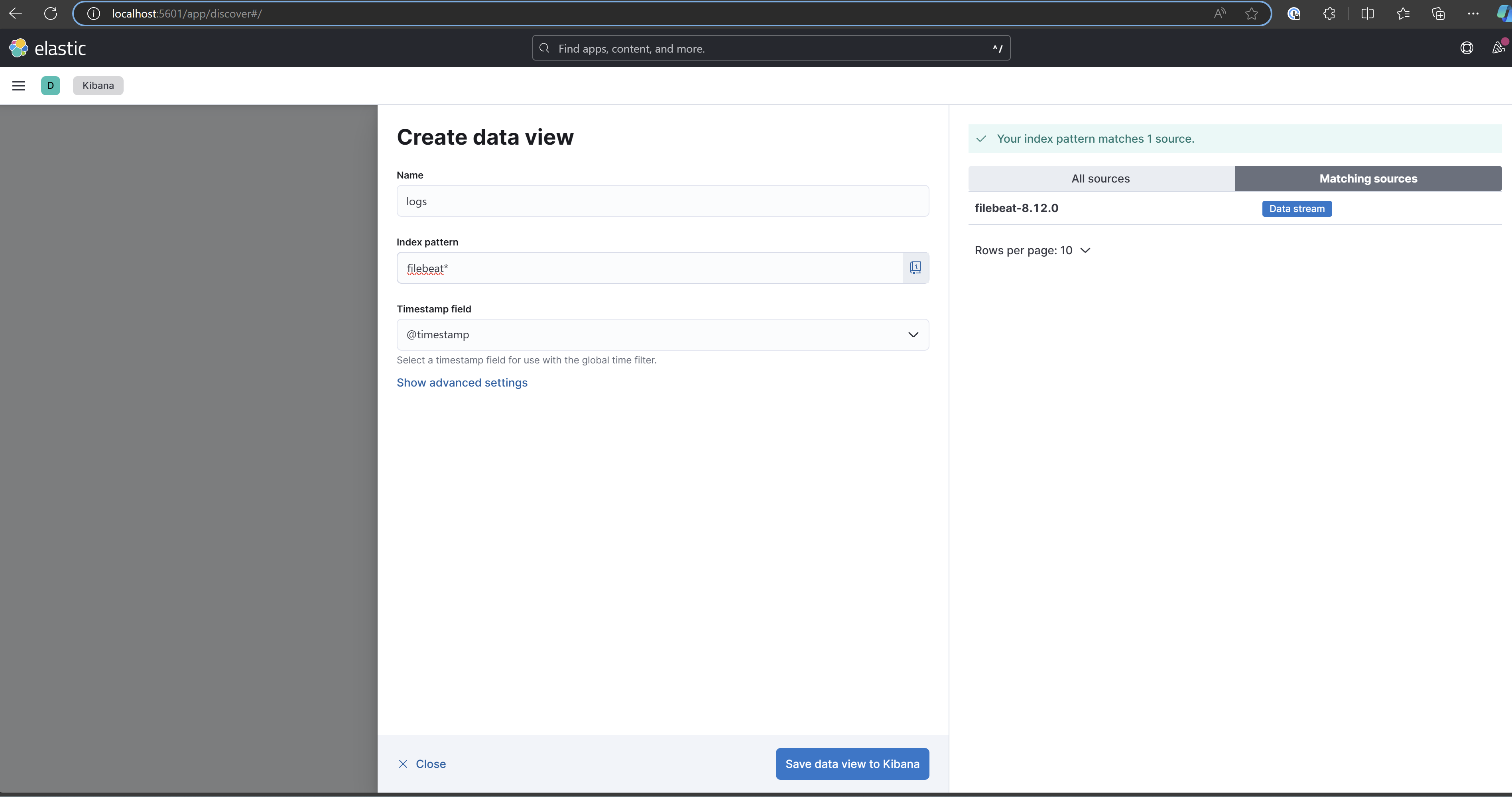
Save the new view, and you will be redirected to the Discover page, where you can view the application logs.

Expand one of the lines by clicking on the arrow on the left side, and you will see all the details of the log. In addition to the message the application logged, you also have all the metadata, such as the logger name, log level, timestamp, and so on.

And the same thing for the exceptions, you have the message logged with the .error log statement plus the stackTrace and the source of the error.

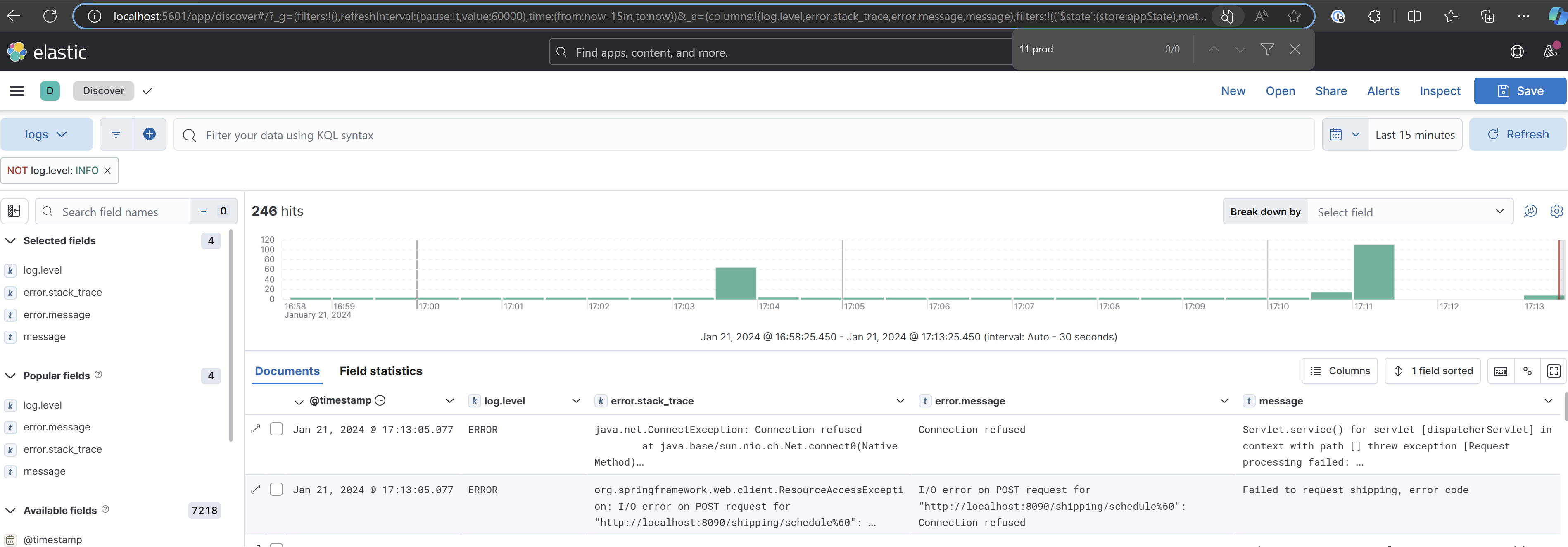
a screenshot of a computer screen with a bar graph

Spend some time familiarizing yourself with Kibana's search syntax, specifically KQL (Kibana Query Language) and Lucene. These powerful query languages enable you to filter and analyze your log data more effectively. For instance, you can try filtering only the Error messages to focus on critical issues.

💡

While exploring Kibana you can keep sending new logs by using the APIs provided.

For more information you can consult the Discover documentation here.

Metrics

Metrics, the second pillar of observability. Metrics are numerical representations that provide valuable insights about the state of a system at any given point in time. We can use these metrics as tools for monitoring and analyzing various aspects of a system's performance, stability, and overall health.

By tracking and evaluating metrics, you can identify trends, patterns, and potential issues within your system, allowing you to make informed decisions and take appropriate actions to optimize performance. Metrics can encompass a wide range of values, such as response times, error rates, resource usage, and throughput, among others.

Let's consider for example the CPU and memory usage. We could naively represent them like this:

{
  "timestamp": "2022-03-15T14:34:30Z",
  "metrics": [
    {
      "label": "cpuUsage",
      "value": 45.3
    },
    {
      "label": "memoryUsage",
      "value": 2048
    }
  ]
}

However, I just created this format, and while it could work, it is not cross-platform compatible and not supported by other libraries or tools, like for example kibana. Instead, we can rely on open and standard tools like Micrometer.

Micrometer is an open-source library for collecting metrics from JVM-based applications. It provides a simple facade over the instrumentation clients for the most popular monitoring systems, allowing you to instrument your JVM-based application code without vendor lock-in. Micrometer also supports a wide range of monitoring systems including Prometheus, Netflix Atlas, Datadog, Elasticsearch and more.

It's important to note that Micrometer is just a facade, it's job is only collecting metrics. To store and visualize them we have to rely in some other system, in this tutorial we chose ElasticSearch and Kibana.

Micrometer - Create metrics

Before starting to create metrics we just have to include the micrometer dependency. For this example I'm using the provided Java Spring Boot API.

<dependency>
  <groupId>io.micrometer</groupId>
  <artifactId>micrometer-registry-elastic</artifactId>
  <version>1.11.2</version>
</dependency>

The next step is to create a MeterRegistry, which is the core component responsible for collecting metrics. Later, we will export all its values to Elastic. Fortunately, Spring Boot already creates a MeterRegistry bean for us and generates some useful metrics, such as CPU load and memory usage (see Spring Actuator).

There are several types of metrics (referred to as meters in Micrometer terminology) that we can create, such as Counters, Distributions, Gauges, and more. I recommend reviewing the Micrometer documentation to gain a better understanding of these metric types, their differences, and typical use cases.

Let's create a metric that counts the number of orders submitted. To accomplish this, we simply need to create the following component:


import io.micrometer.core.instrument.Counter;
import io.micrometer.core.instrument.MeterRegistry;
import org.springframework.stereotype.Component;

@Component
public class OrderServiceMetric {

    private final Counter ordersCounter; (1)

    public OrderServiceMetric(MeterRegistry registry) { (2)
        ordersCounter = Counter.builder("orders.started") (3)
                .description("Counts the number of orders")
                .register(registry);
    }

    public void incrementCounter() {
        ordersCounter.increment(); (4)
    }
}

(1) - We choose the most adequate meter for our use case, in this case a counter

(2) - We register this meter in the global meter registry, it is the meter registry the component responsible to aggregate and export all metrics to Elastic (later chapter).

(3) - We name this counter, this name has to be unique since we are going to use it later to filter and plot the metric.

(4) - We provide a method to increment the counter whenever a order is created

Then we can inject this component on our order service and increment it whenever a order is created:

@Service
public class ClientOrderService {
    .....
    private final OrderServiceMetric orderServiceMetric;

    @Transactional
    public void createOrder(ClientOrderDTO clientOrderDTO) {
        ....
        clientOrderRepository.save(clientOrder);

        orderServiceMetric.incrementCounter();  
      .....
    }
}

💡

The previous classes are just an example, in a real scenario the metric component shouldn't be injected in the service. We can think in a cleaner way to do it, like using AOP for example.

And that's it—the metric is created and stored in the MeterRegistry. Now let's see how to send it to Elasticsearch.

Export metrics to Elastic

This is quite simple, just add the following properties to your application.properties

management.elastic.metrics.export.host=http://localhost:9200 (1)
management.elastic.metrics.export.index=demo-metrics         (2)
management.elastic.metrics.export.step=15s                   (3)
management.endpoints.web.exposure.include=*                  (4)

(1) - We define where our ElasticSearch server is. Don't forget to adapt the hostname to your environment

(2) - We define to which index we send the metrics

(3) - We export the metrics to Elastic every 15seconds

(4) - As said, spring actuator creates some metrics for us, here we say that we want to expose them all in the actuator endpoints

With this configuration, the metrics will be automatically sent to Elasticsearch every 15 seconds. Just ensure that all components are running by checking the Docker Compose from the previous section.

Kibana - Create dashboards

Now that the metrics are being ingested by Elasticsearch, we can create dashboards to display our metrics graphically. However, before doing so, we need to create a new data view in Kibana for the metrics indexes (as we did for the logs).

Again on Kibana Discover section click on "Create Data View"

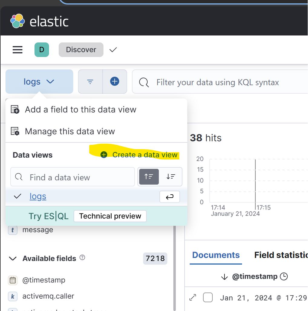
As done in the logs chapter, create a new data view, this time with the name "metrics" and the index pattern "metrics*"

If you play a bit with the columns of the table you can see that we have a lot of metrics. We see for example jvm threads, hikari, cpu usage...

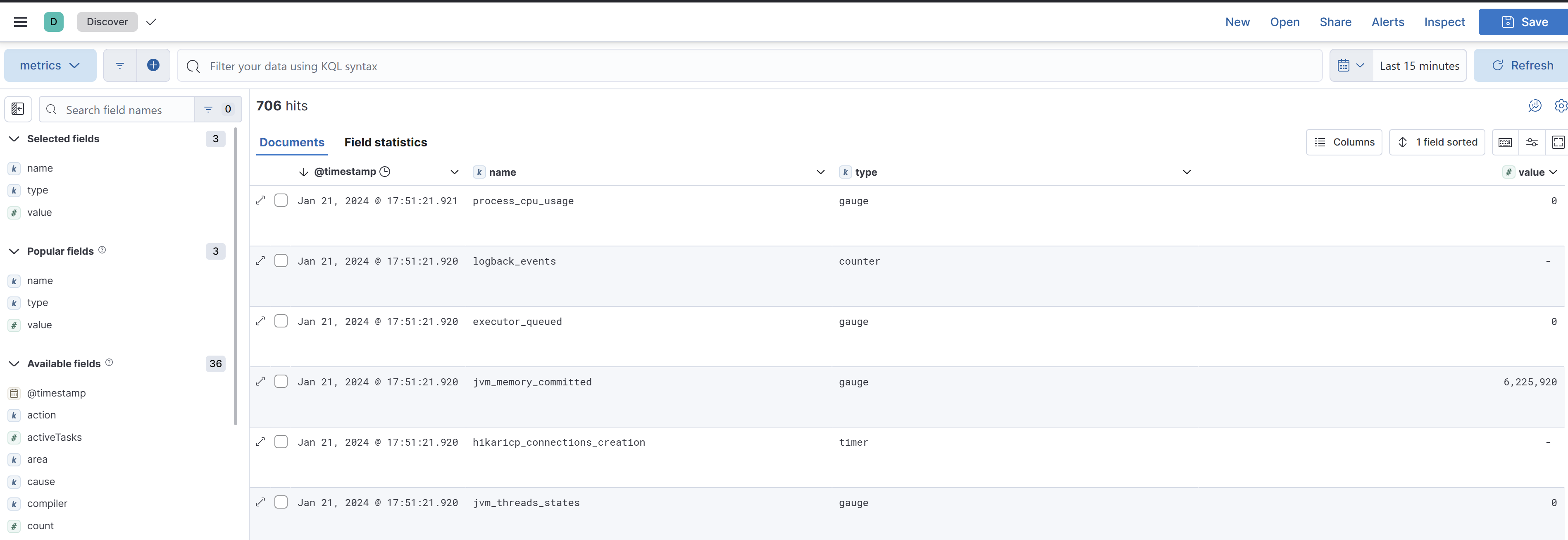
We are seeing only the spring actuator metrics, our custom metric is only created when a order is created, so let's create some orders. To do so, send some POST requests to the /orders endpoint

POST http://localhost:8080/orders
Content-Type: application/json

{
  "clientName": "John Doe",
  "products": [
    {
      "id": 1,
      "quantity": 2
    },
    {
      "id": 3,
      "quantity": 1
    }
  ]
}

After sending a few requests, you should begin to see the custom metric appear in Kibana as well. Remember that the metrics are sent every 15 seconds, a small delay is expected.

With the metrics now on Elastic, we can now start creating some visualizations. Navigate to:

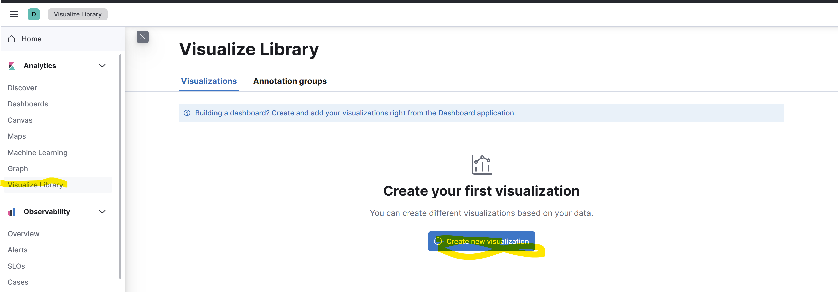
After clicking on the Create new visualization button you will be asked what type of visualization you want to create, for this tutorial we choose Lens.

To start just define the X axis as the timestamp and the Y axis as the Value. To do this just drag and drop the column names from the left side to the right side

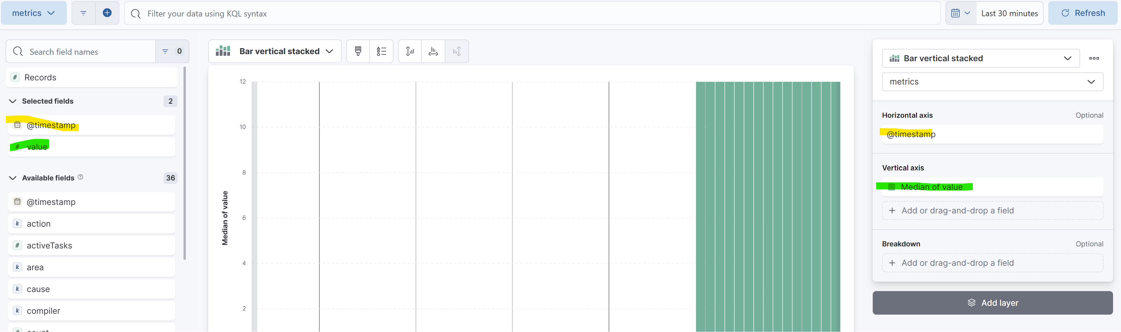
Then click on the "Median of value" to edit its settings:

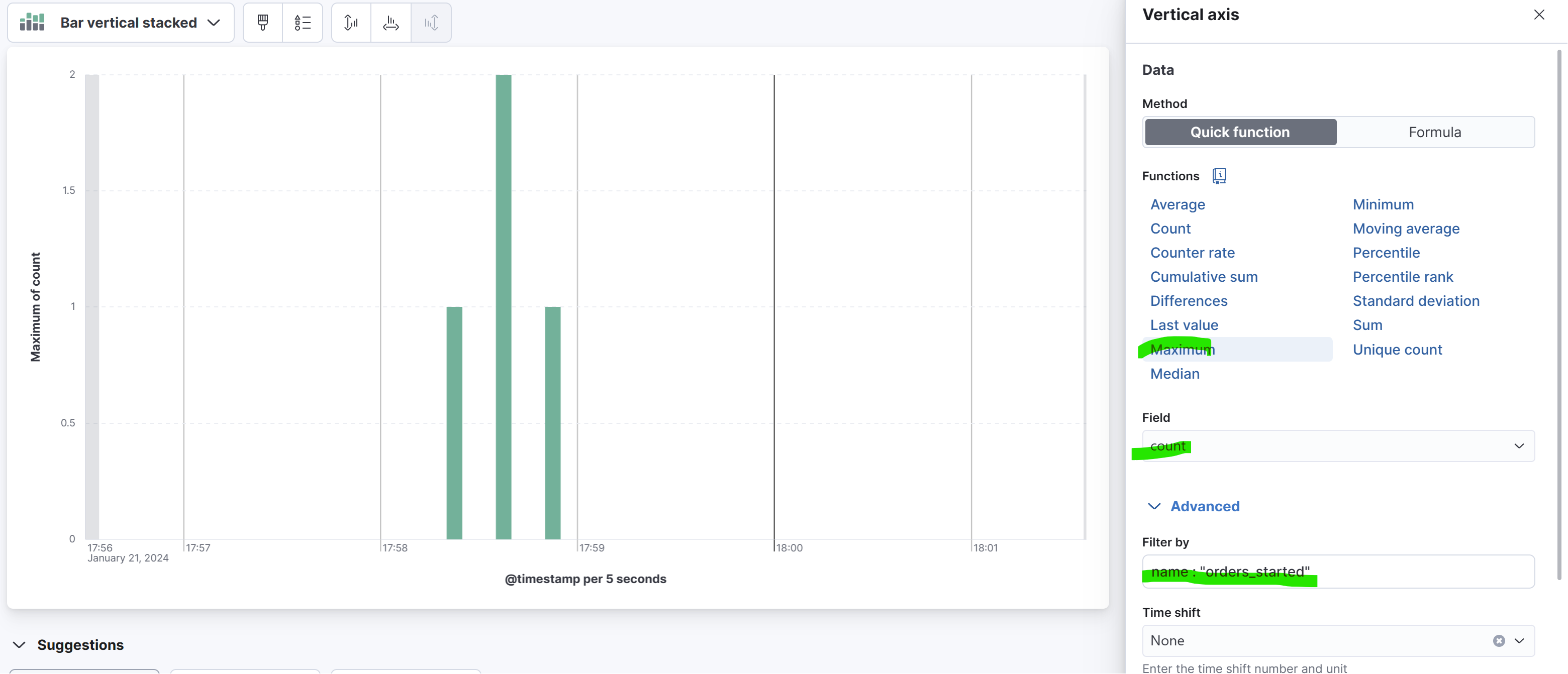
Here, we are plotting the maximum value of the count property for the metric named orders_started. Upon inspecting the metric, we can see that the value of the count is stored in a property called count. However, other types of metrics have different properties, such as mean, max, and so on. Since we can have multiple metrics for a period of time, as shown in the previous screenshot with 5-second buckets, we need to decide how to aggregate them. In this case, we chose the Maximum function. To learn more about these aggregations you can check the Kibana documentation here.

💡

To check which properties a metric can contain consult the micrometer documentation.

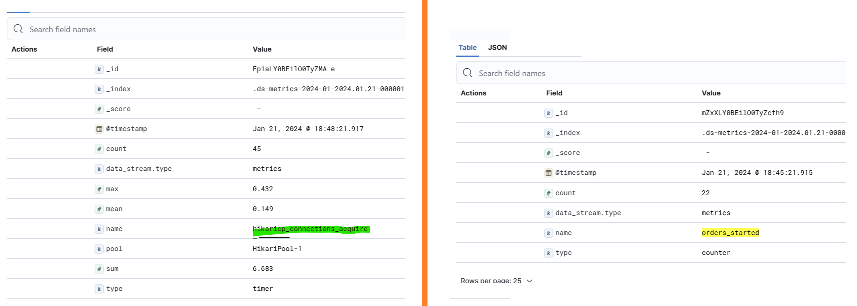
As seen in the next picture, each metric type can contain different properties.

On the left we have a timer, that contains the count, max, mean, sum values, and on the right we have a counter that contains a single value, the count.

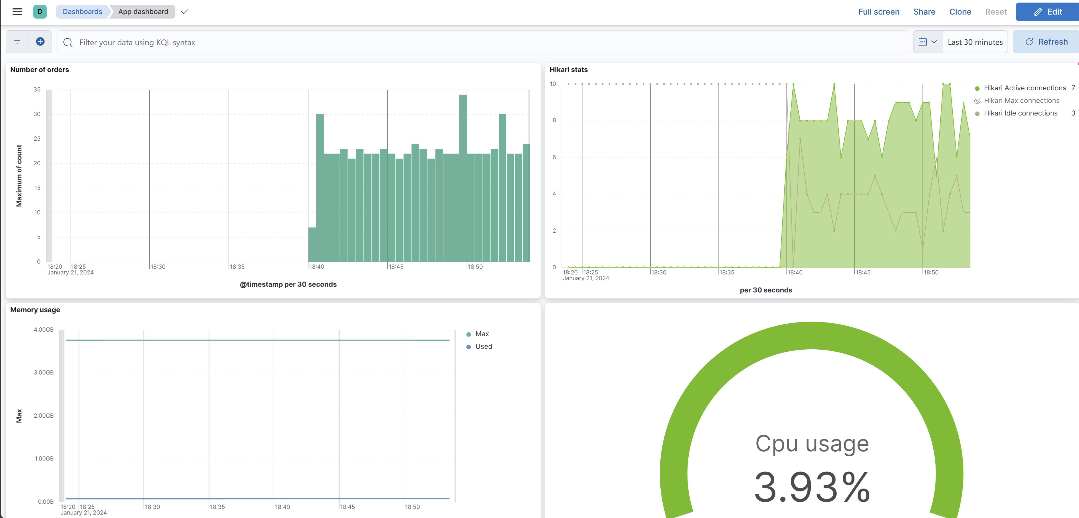
After playing a bit with the dashboard and visualizations you should be able to create dashboards like the following.

Kibana dashboard

Tracing

Tracing, the third pillar of observability, and perhaps the most complex to implement. The purpose of tracing, is to see how a transaction or request moves through a system. It is especially useful in distributed systems composed of multiple independent applications. As we are going to see, traces are basically the logs related with a specific transaction (a bit of simplification here). We could rely on Kibana, as we saw before, however how can we related the logs from Application A with Application B? Typically in distributed systems the transaction goes through multiple systems, and we have millions of other transactions running at the same time.

Although our primary focus is on the ELK stack, it's worth mentioning the OpenTelemetry standard.

OpenTelemetry is an Observability framework and toolkit designed to create and manage telemetry data such as traces, metrics, and logs. *What is OpenTelemetry? | OpenTelemetry

In this tutorial, we won't be using OpenTelemetry or the OpenTelemetry bridge for APM. However, the fundamental concepts behind APM are not unfamiliar to the OpenTelemetry standard.

And what is specifically Elastic APM (Application Performance Monitoring)?

Elastic APM is an application performance monitoring system built on the Elastic Stack. It allows you to monitor software services and applications in real time, by collecting detailed performance information on response time for incoming requests, database queries, calls to caches, external HTTP requests, and more. This makes it easy to pinpoint and fix performance problems quickly.
*Application performance monitoring (APM) | Elastic Observability [8.12] | Elastic

Basically APM is the tool that will instrument our code, collect metrics, add the necessary metadata to define spans and send everything to elastic. This information is then aggregated and can be visualized in Kibana.

Let's start by define some concepts required to define a trace.

Trace: A trace represents the entire journey of a single request as it moves through a distributed system. It's a collection of one or more spans.
Span: A span is the primary building block of a trace. It represents a specific unit of work done in a system, like a function call or a database query. Each span contains details about the operation it represents, such as its name, duration, and status.
Transaction: Transactions are a special kind of span that have additional attributes associated with them. They describe an event captured by an Elastic APM agent instrumenting a service. The transaction is specific to APM, it is not part of OpenTelemetry. When using the OpenTelemetry bridge the transactions are simply converted to a span.
Trace ID and Span ID: Each trace and span have a unique identifier. These IDs are crucial for correlating the parts of a trace across different services and logs. It is very important that these traceID is propagated with the request along the system.
Span attributes: All the metadata associated with a span, for example if it the span represents a database query, the attributes can contain the query and the execution time.

If we represent a trace using a diagram we get something like the follwoing:

With this visual representation of a trace we can easily see the full lifecycle of a transaction, in this example a order. By representing the trace along the time it is also very easy to visualize where a bottleneck may be.

In addition to the timings, appending metadata to the spans provides even more details about the specific unit of work for each span. For instance, with SQL queries, having the query directly in the trace makes troubleshooting slow queries faster. Similarly, for HTTP calls, it's helpful to include the URL and response time in the span.

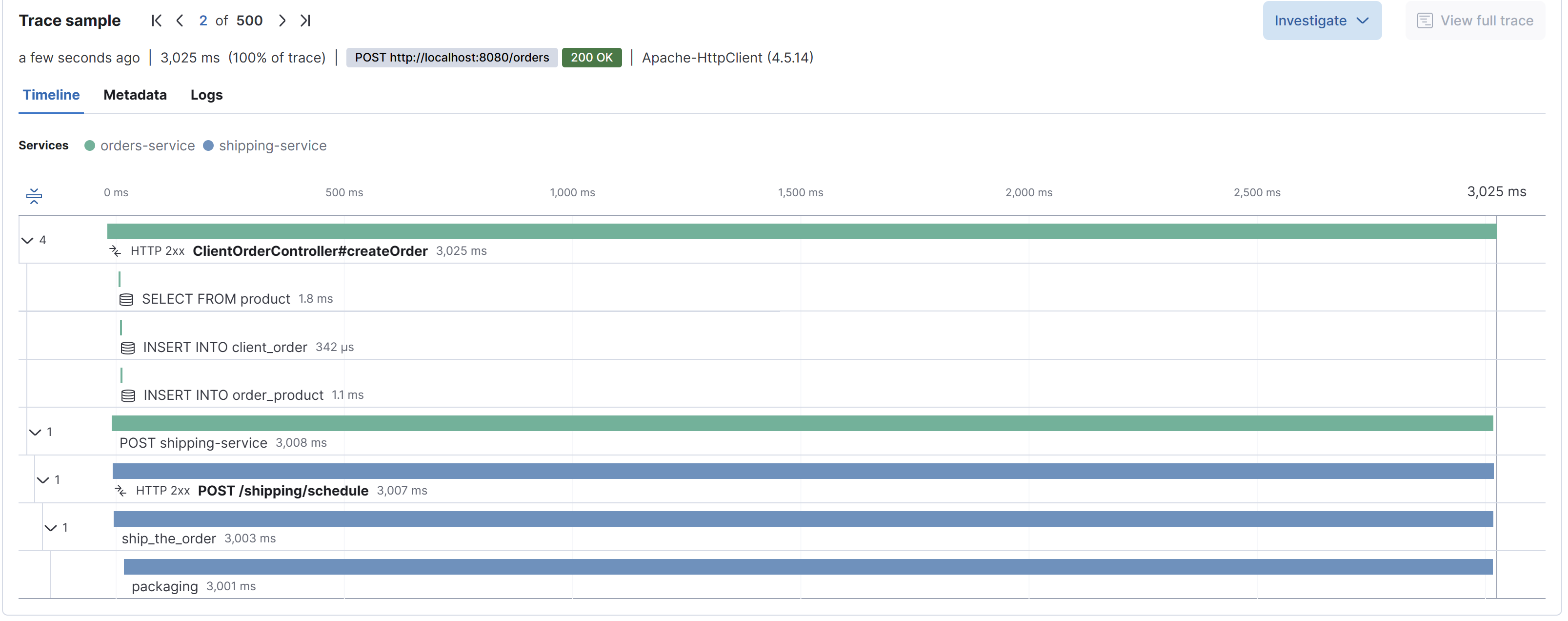
Kibana visual representations of traces is very similar to the previous image:

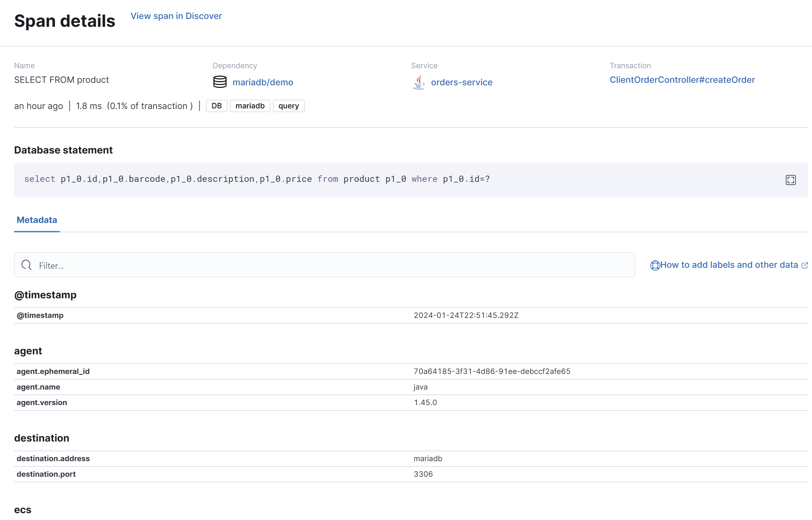
And if we click each span we can get all the details attached to it:

How are traces propagated across different services?

But how does APM correlate events in different services? Keep in mind that these two services are completely independent, and they even have different stacks—one is written in Java and the other in Python.

The magic is in a specific header injected on each HTTP request. The full details about this header are in W3C Trace Context specification here, but let's analyze the headers that the shipping service is receiving.

Elastic-Apm-Traceparent: 00-723ce8c809c8e2e249d5a00fdf1bb2d5-41f8915f37507605-01
Traceparent: 00-723ce8c809c8e2e249d5a00fdf1bb2d5-41f8915f37507605-01

We see that we have 2 distinct headers with the same value. Let's discard the Elastic-Apm-Traceparent. This header was used by the older versions of APM, now it is only kept for backward compatibility purposes. The most recent versions of APM use the traceparent as it is defined in the W3C Trace Context specification. This increases the compatibility with other tracing libraries.

The APM agent, or any other tracing library compliant with the W3C Trace Context specification, running on the target application uses this header to determine whether to create a new trace or continue being part of the existing one. Then each tracing library is responsible to send the spans they collect to the central application performance monitoring tool, in our case Kibana/APM.

By looking to the header value it is clear that it contains some encoded information.

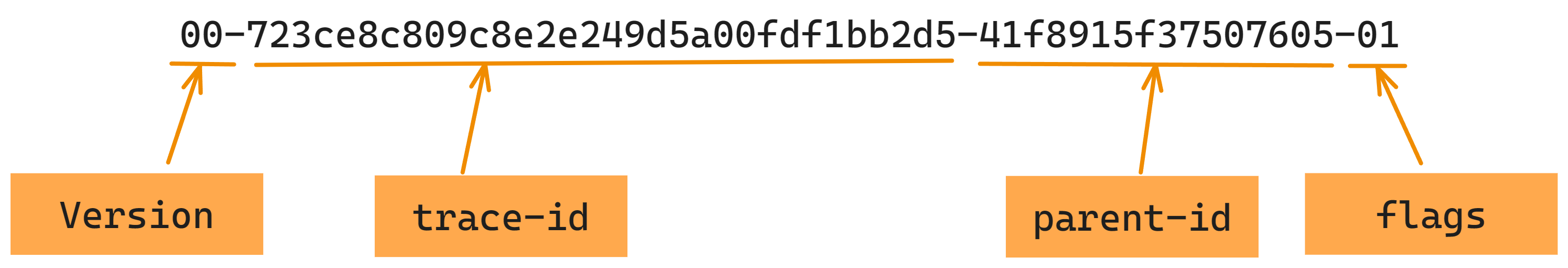
The version identifies the format version we are receiving. As the name suggests, the trace-id identifies the trace, and the parent-id represents the parent span id. These are the same concepts we saw at the beginning of this chapter. Finally we have the flags, this value is not currently used by APM.

And this is the key to achieving distributed tracing: the context of the trace must be passed to each service in the flow. It doesn't matter if it's an HTTP API, a Kafka Topic, or a ServiceBus. If one service in the chain stops propagating the traceparent header, the trace will end there, and a new one will be created afterward.

Conclusion

In this post, we demonstrated how to implement the three pillars of observability using tools from the ELK stack, which includes Elasticsearch, Logstash, Kibana and APM. However, it's important to note that there are numerous other tools available, including open-source alternatives, that can be used to achieve similar results. The concepts and methodologies we employed with the ELK stack can be applied to other tools as well, making it possible to adapt this approach to a variety of different environments and technology stacks.

The key takeaway is that, regardless of the tools chosen, it is essential to have a robust observability infrastructure in place to ensure a healthy and high-performing distributed system.

💡

All source code available here: https://github.com/hugo-ma-alves/distributed-tracing-demo